There are several issues here that should be mentioned:
i) chi-squared tests of goodness of fit tend to have very low power. There are much better alternatives
ii) if you don't have a completely specified distribution, but the parameters are estimated efficiently on the full data set (rather than the grouped data) - for example, if we're looking at residuals in an ANOVA - then the chi-square statistic doesn't actually have a chi-square distribution.
iii) if the point is to assess the assumptions of some other procedure, formal goodness of fit testing is not really answering the right question.
If it's made sufficiently clear what we're testing - (a) raw data or residuals, and (b) if raw data whether it's with specified parameters or estimated parameters - then I can describe how to go about it.
Population parameters are specified in advance
If the parameters are all specified in advance, then you divide the data into bins. Your linked extract indicated one way to do this, which is to divide the data up into equal sized bins via the inverse cdf.
$F^{-1}(p)$ ($\,=\Phi^{-1}(p)$ for a standard normal) cuts off $p$ of the probability to its left. So by taking $p_i = 0.25,0.5,0.75$ you'd get 4 bins. In this case (n=50) slightly more bins would be better (say $k=6$, or perhaps $8$), but the idea of taking regions so that you get equal or near equal expected counts is good.
Then count the number of observations in each bin, $O_i, i=1,2,...,k$. The expected count $E_i=np_i$ (which $=n/k$ when the proportions are equal).
Then you compute $\sum_{i=1}^k \frac{(O_i-E_i)^2}{E_i}$ and this will have an approximately chi-squared distribution with $k-1$ degrees of freedom; you lose 1 because the expected total is set equal to the observed total. (So with 4 groups, that's 3 d.f.)
Population parameters are (efficiently) estimated from the grouped data
In this case, you don't have the raw data - it's already been grouped before the parameters were estimated (such estimation via MLE is often not simple - EM is sometimes used, but minimum chi-square estimation will work quite well for this purpose and may be easier to carry out).
The $p_i$ and hence expected values are calculated based on those estimated parameters.
Calculation then proceeds much as before, except you lose one additional degree of freedom per parameter estimated. So in this case, with 4 groups and 2 parameters, you'd have 1 d.f. left.
Parameters are efficiently estimated on the ungrouped data
This includes the case where the data have been standardized by the sample estimates. This works much as case 2. above, except that you no longer have an asymptotic chi-square distribution for the test statistic under the null hypothesis.
This has long been known, but many elementary treatments of the chi-squared goodness of fit test seem completely ignorant of it. See the excellent discussion here for some illustration and further explanation.
However, the distribution is bounded between $\chi^2_{k-1}$ and $\chi^2_{k-p-1}$ where $p$ parameters are estimated, so you can get bounds on p-values. Alternatively, you can perform simulation to work out either critical values or p-values.
If the group boundaries are estimated from the data, this apparently doesn't affect the asymptotic distribution (so if $n$ is large you can pretty much ignore that, though if you're basing your null distribution off simulation, you'd be able to include any effect it might have, even in small samples)
So now, to your data. I assume we're in situation 3. I'll pull your data into R and do the calculations step-by-step (in the way one might do if hand calculation were ever necessary). I scanned your data into y:
> mean(y)
[1] -0.1646
> sd(y)
[1] 1.16723
Find bin boundaries (proceeds as in the example in your linked document):
> mean(y)+sd(y)*qnorm((0:4)/4)
[1]       -Inf -0.9518845 -0.1646000  0.6226845        Inf
Here -Inf (=$-\infty$) is the left 'limit' of the lower bin and Inf ($\infty$) is the right limit of the upper bin.
Count how many in each bin:
> table(cut(y,mean(y)+sd(y)*qnorm((0:4)/4)))

  (-Inf,-0.952] (-0.952,-0.165]  (-0.165,0.623]    (0.623, Inf]
             14              11              14              11
Let's put that in something:
> Oi = table(cut(y,mean(y)+sd(y)*qnorm((0:4)/4)))
The expected number in each bin, $E_i=np_i$ is $n/k$ = 50/4 = 12.5.
> Ei = 50/4
Calculate the statistic:
> sum((Oi-Ei)^2/Ei)
[1] 0.72
and this has a distribution function that lies between a $\chi^2_1$ and $\chi^2_3$. There's no need to proceed, since the statistic is smaller than the expectation for 1.d.f (it simply won't reject, since the p-value is already more than 0.3). But let's calculate anyway:
> pchisq(sum((Oi-Ei)^2/Ei),1,lower.tail=FALSE)
[1] 0.3961439
> pchisq(sum((Oi-Ei)^2/Ei),3,lower.tail=FALSE)
[1] 0.86849
So the p-value is above 0.40 but below 0.87.
However, since we could only be sure we could reject if the higher number was below the significance, level, we can just plug the $O_i$'s into a chi-square test:
> chisq.test(Oi)

        Chi-squared test for given probabilities

data:  Oi
X-squared = 0.72, df = 3, p-value = 0.8685
We get the upper bound on the p-value. If that was below your significance level, you could reject.
--
If we did simulation:
res = replicate(100000,{x=rnorm(50);
                     Oi = table(cut(x,mean(x)+sd(x)*qnorm((0:4)/4)));
                     sum((Oi-Ei)^2/Ei)})
> sum(res>=0.72)/length(res)
[1] 0.76827
We get a p-value of 0.77. (This only takes a couple of seconds.)
If you must test normality, a Shapiro-Wilk test would be better:
> shapiro.test(y)

        Shapiro-Wilk normality test

data:  y
W = 0.9448, p-value = 0.02092
But in many cases, a Q-Q plot is probably more use than a formal hypothesis test:
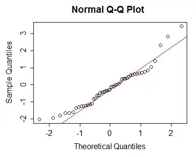
because we can assess the kind and extent of the deviation from normality fairly readily - the left tail is "short", the right tail is somewhat "long" ... i.e. the data are mildly right skew. [Would this amount of skewness matter? For things like t-tests or regression or ANOVA, not very much -- but in any of those cases, the assumption relates to the conditional distribution, not the marginal, so you must be careful to check the right quantities.]