Computing mathematical expectation of the correlation coefficient or $R^2$ in linear regression

Question

I'm re-posting a question from math.stackexchange.com, I think the current answer in math.se is not right.

Select $n$ numbers from a set $\{1,2,...,U\}$, $y_i$ is the $i$th number selected, and $x_i$ is the rank of $y_i$ in the $n$ numbers. The selection is without replacement. $n$ is always smaller than $U$. The rank is the order of the a number after the $n$ numbers are sorted in ascending order.

We can get $n$ data points $(x_1, y_1), (x_2, y_2), ..., (x_n, y_n)$, And a best fit line for these data points can be found by linear regression. $r_{xy}$ (correlation coefficient) is the goodness of the fit line, I want to calculate $\mathbb{E}(r_{xy})$ or $\mathbb{E}(r_{xy}^2)$ (correlation of determination).

If the $\mathbb{E}[r_{xy}]$ cannot be calculated, an estimation or lower bound is still OK.

Updated: By calculating the sample correlation coefficient using randomly generated data, we can see that $r_{xy}$ is quite closed to 1, so I want to proof it from the theoretical view, or theoretically say the data generated by the above method is very linear.

Updated: Is it possible to get the distribution of sample correlation coefficient?

Answer 1

If you only want to show $r^2_{xy}$ must be close to 1, and compute a lower bound for it, it's straightforward, because that means for given $U$ and $n$ you only need to maximize the variance of the residuals. This can be done in exactly four symmetric ways. The two extremes (lowest and highest possible correlations) are illustrated for $U=20, n=9$.

For large values of $U$ and appropriate values of $n$, $r^2_{xy}$ can actually get close to 0. For example, with $n=100$ and very large values of $U \gg n$, $r^2_{xy} \sim 0.03$ in the worst case.

Answer 2

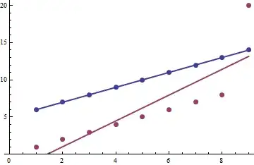
Re-arrange the problem in terms of new variables, so that $1\leq z_1<z_2<\dots<z_n\leq U$. Then we have $(x_i,y_i)=(x_i,z_{x_i})$, as @whuber pointed out in the comments. Thus you are effectively regressing $z_j$ on $j$, and $r_{xy}=r_{xz}$. Thus if we can work out the marginal distribution for $z_j$, and show that it is basically linear in $j$ the problem is done, and we will have $r_{xy}\sim 1$.

We first need the joint distribution for $z_1,\dots,z_n$. This is quite simple, after you have the solution, but I found it not straight forward before I did the maths. Just a brief lesson in doing maths paying off - so I will present the maths first, then the easy answer.

Now, the original joint distribution is $p(y_1,\dots,y_n)\propto 1$. Changing variables simply relabel things for discrete probabilities, and so the probability is still constant. However, the labelling is not 1-to-1, thus we can't simply write $p(z_1,\dots,z_n)=\frac{(U-n)!}{U!}$. Instead, we have

$$\begin{array}\\p(z_1,\dots,z_n)=\frac{1}{C} & 1\leq z_1<z_2<\dots<z_n\leq U\end{array}$$

And we can find $C$ by normalisation $$C=\sum_{z_n=n}^{U}\sum_{z_{n-1}=n-1}^{z_n-1}\dots\sum_{z_2=2}^{z_3-1}\sum_{z_1=1}^{z_2-1}(1)=\sum_{z_n=n}^{U}\sum_{z_{n-1}=n-1}^{z_n-1}\dots\sum_{z_2=2}^{z_3-1}(z_2-1)$$ $$=\sum_{z_n=n}^{U}\sum_{z_{n-1}=n-1}^{z_n-1}\dots\sum_{z_3=2}^{z_4-1}\frac{(z_3-1)(z_3-2)}{2}=\sum_{z_n=n}^{U}\dots\sum_{z_4=4}^{z_5-1}\frac{(z_4-1)(z_4-2)(z_4-3)}{(2)(3)}$$ $$=\sum_{z_n=n}^{U}\sum_{z_{n-1}=n-1}^{z_n-1}\dots\sum_{z_{j}=j}^{z_{j+1}-1}{z_j-1 \choose j-1}={U \choose n}$$

Which shows the relabeling ratio is equal to $\frac{(U-n)!}{U!}{U \choose n}=\frac{1}{n!}$ - for each $(z_1,\dots,z_n)$ there is $n!$ $(y_1,\dots,y_n)$ values. Makes sense because any permutation of the lables on $y_i$ leads to the same set of ranked $z_i$ values. Now, the marginal distribution $z_1$, we repeat above but with the sum over $z_1$ dropped, and a different range of summation for the remainder, namely, the minimums change from $(2,\dots,n)$ to $(z_1+1,\dots,z_1+n-1)$, and we get:

$$p(z_1)=\sum_{z_n=z_1+n-1}^{U}\;\;\sum_{z_{n-1}=z_1+n-2}^{z_n-1}\dots\sum_{z_2=z_1+1}^{z_3-1}p(z_1,z_2,\dots,z_n)=\frac{{U-z_1 \choose n-1}}{{U \choose n}}$$

With support $z_1\in\{1,2,\dots,U+1-n\}$. This form, combined with a bit of intuition shows that the marginal distribution of any $z_j$ can be reasoned out by:

1. choosing $j-1$ values below $z_j$, which can be done in ${z_j-1\choose j-1}$ ways (if $z_j\geq j$);
2. choosing the value $z_j$, which can be done 1 way; and
3. choosing $n-j$ values above $z_j$ which can be done in ${U-z_j\choose n-j}$ ways (if $z_j\leq U+j-n$)

This method of reasoning will effortly generalise to joint distributions, such as $p(z_j,z_k)$ (which can be used to calculate the expected value of the sample covariance if you want). Hence we have:

$$\begin{array}{c c}\\p(z_j)=\frac{{z_j-1\choose j-1}{U-z_j\choose n-j}}{{U \choose n}} & j\leq z_j\leq U+j-n \\p(z_j,z_k)=\frac{{z_j-1\choose j-1}{z_k-z_j-1 \choose k-j-1}{U-z_k\choose n-k}}{{U \choose n}} & j\leq z_j\leq z_k+j-k\leq U+j-n \end{array}$$

Now the marginal is the pdf of a negative hypergeometric distribution with parameters $k=j,r=n,N=U$ (in terms of the paper's notation). Now this is clear not linear exactly in $j$, but the marginal expectation for $z_j$ is

$$E(z_j)=j\frac{U+1}{n+1}$$

This is indeed linear in $j$, and you would expect beta coefficient of $\frac{U+1}{n+1}$ from the regression, and intercept of zero.

UPDATE

I stopped my answer a bit short before. Have now completed hopefully a more complete answer

Letting $\overline{j}=\frac{n+1}{2}$, and $\overline{z}=\frac{1}{n}\sum_{j=1}^{n}z_j$, the expected square of the sample covariance between $j$ and $z_j$ is given by:

$$E[s_{xz}^2]=E\left[\frac{1}{n}\sum_{j=1}^{n}(j-\overline{j})(z_j-\overline{z})\right]^2$$ $$=\frac{1}{n^2}\left[\sum_{j=1}^{n}(j-\overline{j})^2E(z_j^2)+2\sum_{k=2}^{n}\sum_{j=1}^{k-1}(j-\overline{j})(k-\overline{j})E(z_jz_k)\right]$$

So we need $E(z_j^2)=V(z_j)+E(z_j)^2=Aj^2+Bj$, where $A=\frac{(U+1)(U+2)}{(n+1)(n+2)}$ and $B=\frac{(U+1)(U-n)}{(n+1)(n+2)}$ (using the formula in the pdf file). So the first sum becomes

$$\sum_{j=1}^{n}(j-\overline{j})^2E(z_j^2)=\sum_{j=1}^{n}(j^2-2j\overline{j}+\overline{j}^2)(Aj^2+Bj)$$ $$=\frac{n(n-1)(U+1)}{120}\bigg( U(2n+1)+(3n-1)\bigg)$$

We also need $E(z_jz_k)=E[z_j(z_k-z_j)]+E(z_j^2)$.

$$E[z_j(z_k-z_j)]=\sum_{z_k=k}^{U+k-n}\sum_{z_j=j}^{z_k+j-k}z_j(z_k-z_j) p(z_j,z_k)$$ $$=j(k-j)\sum_{z_k=k}^{U+k-n}\sum_{z_j=j}^{z_k+j-k}\frac{{z_j\choose j}{z_k-z_j \choose k-j}{U-z_k\choose n-k}}{{U \choose n}}=j(k-j)\sum_{z_k=k}^{U+k-n}\frac{{z_k+1 \choose k+1}{U+1-(z_k+1)\choose n-k}}{{U \choose n}}$$ $$=j(k-j)\frac{{U+1\choose n+1}}{{U \choose n}}=j(k-j)\frac{U+1}{n+1}$$ $$\implies E(z_jz_k)=jk\frac{U+1}{n+1}+j^2\frac{(U+1)(U-n)}{(n+1)(n+2)}+j\frac{(U+1)(U-n)}{(n+1)(n+2)}$$

And the second sum is:

$$2\sum_{k=2}^{n}\sum_{j=1}^{k-1}(j-\overline{j})(k-\overline{j})E(z_jz_k)$$ $$=\frac{n(U+1)(n-1)}{720(n+2)}\bigg(6(U-n)(n^3-2n^2-9n-2) + (n+2)(5 n^3- 24 n^2- 35 n +6)\bigg)$$

And so after some rather tedious manipulations, you get for the expected value of the squared covariance of:

$$E[s_{xz}^2]=\frac{(n-1)(n-2)U(U+1)}{120}-\frac{(U+1)(n-1)(n^3+2n^2+11n+22)}{720(n+2)}$$

Now if we have $U>>n$, then the first term dominates as it is $O(U^2n^2)$, whereas the second term is $O(Un^3)$. We can show that the dominant term is well approximated by $E[s_{x}^2s_{z}^2]$, and we have another theoretical reason why the pearson correlation is very close to $1$ (beyond the fact that $E(z_j)\propto j$).

Now the expected sample variance of $j$ is just the sample variance, which is $s_x^2=\frac{1}{n}\sum_{j=1}^{n}(j-\overline{j})^2=\frac{(n+1)(n-1)}{12}$. The expected sample variance for $z_j$ is given by:

$$E[s_z^2]=E\left[\frac{1}{n}\sum_{j=1}^{n}(z_j-\overline{z})^2\right]=\frac{1}{n}\sum_{j=1}^{n}E(z_j^2)-\left[\frac{1}{n}\sum_{j=1}^{n}E(z_j)\right]^2$$ $$=\frac{A(n+1)(2n+1)}{6}+\frac{B(n+1)}{2}-\frac{(U+1)^2}{4}$$ $$=\frac{(U+1)(U-1)}{12}$$

Combining everything together, and noting that $E[s_x^2s_z^2]=s_x^2E[s_z^2]$, we have:

$$E[s_x^2s_z^2]=\frac{(n+1)(n-1)(U+1)(U-1)}{144}\approx \frac{(n-1)(n-2)U(U+1)}{120}\approx E[s_{xz}^2]$$

Which is approximately the same thing as $E[r_{xz}^2]\approx 1$