Confusion between caret randomForest predict() results and reported model performance

Question

This question seems related, but the consensus was that the issue had to do scaling the data, which I do prior to training, so I don't think that's the issue:

• Issue on prediction with FinalModel of RandomForest in R using the CARET package

I've uploaded a sample data set, and here is how I generated my model:

library(randomForest)
library(caret)
library(ggplot2)

data <- read.csv("http://pastebin.com/raw.php?i=mE5JL1dm")

data_pred <- data[, 1:(ncol(data) - 1)]
data_resp <- as.factor(data$y)

data_trans <- preProcess(data_pred, method = c("center", "scale"))
data_pred_scale <- predict(data_trans, data_pred)

trControl <- trainControl(method = "LGOCV", p = 0.9, savePredictions = T)

set.seed(123)
model <- train(x = data_pred_scale, y = data_resp,
               method = "rf", scale = F,
               trControl = trControl)

Here's what caret() reports as the model performance:

> model

Random Forest 

516 samples
 11 predictors
  5 classes: '0', '0.5', '1', '1.5', '2' 

No pre-processing
Resampling: Repeated Train/Test Splits Estimated (25 reps, 0.9%) 

Summary of sample sizes: 468, 468, 468, 468, 468, 468, ... 

Resampling results across tuning parameters:

  mtry  Accuracy  Kappa  Accuracy SD  Kappa SD
  2     0.747     0.663  0.0643       0.0853  
  6     0.76      0.68   0.0507       0.068   
  11    0.758     0.678  0.0574       0.0763  

Accuracy was used to select the optimal model using  the largest value.
The final value used for the model was mtry = 6. 

In my "real" model, I have a training/hold-out set, and creating two sets of plots showing model predictions for the training/hold-out sets vs. the corresponding true observations. That's when I noticed something that seemed odd to me.

# data set of model predictions on training data vs. actual observations
results <- data.frame(pred = predict(model, data_pred_scale),
                      obs = data_resp)

table(results)

     obs
pred    0 0.5   1 1.5   2
  0   148   0   0   0   0
  0.5   0 132   0   0   0
  1     0   0 139   0   0
  1.5   0   0   0  38   0
  2     0   0   0   0  59

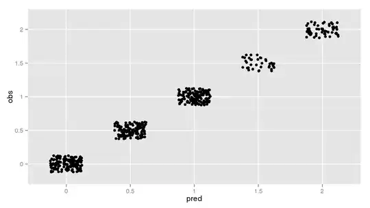
And here's a plot confirming 100% accuracy on the training set:

p <- ggplot(results, aes(x = pred, y = obs))
p <- p + geom_jitter(position = position_jitter(width = 0.25, height = 0.25))
p

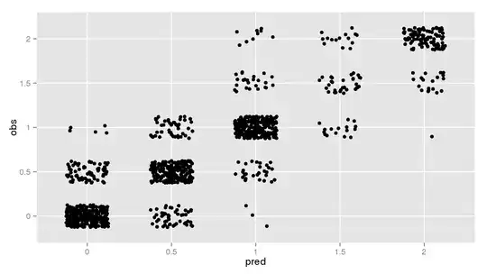
But if I look at the saved tuning predictions, subsetting only those where mtry = 6 (what caret reports as the final model), I don't get anywhere near that performance:

model_resamples <- model$pred[model$pred$mtry == 6, c("pred", "obs")

table(model_resamples)

        0 0.5   1 1.5   2
  0   296  69   5   0   0
  0.5  51 228  48   0   0
  1     3  28 255  24   9
  1.5   0   0  16  32  15
  2     0   0   1  19 101

And the same sort of plot:

p <- ggplot(model_resamples, aes(x = pred, y = obs))
p <- p + geom_jitter(position = position_jitter(width = 0.25, height = 0.25))
p

Is this just a case of over-fitting where holding out 10% of the data can create a 25% decrease in performance, yet the final model trained with the same parameters but all rows can yield 100% performance? It seemed unlikely, but that's the only thing coming to mind at the moment.

I just want to make sure there's nothing wrong in my training or predicting methods where I'm creating a problem where there shouldn't be one.

---

Note: I created the tables/plots prior to adding set.seed() in the model training code above. The exact table and plot may differ slightly, but in re-running, they general result is the same (perfect re-prediction vs. ~77% reported by the model). It didn't seem to warrant re-doing the results/plots above, so I left them.

Answer 1

The summary printed for the model contains the line

6     0.76      0.68   0.0507       0.068   

which tells you that the expected/average accuracy for a proprley cross-validaded (training separated from testing) experiment should be 0.76

I have never used the line

model$pred[model$pred$mtry == 6, c("pred", "obs") 

before but I guess it is giving you the aggregated results of all the internal cross-validations done when testing for mtry=6. You get a 0.7893916 which is pretty close to 0.76.

Caret, by default also generates the final model with all the training data provided, which is the model used in the line

pred=predict(model, data_pred_scale),

so what is curious is that the random forest generated gets a 100% accuracy when tested with the data used to train it. It is not impossible, of course, but just curious.

This phenomenon is not technically called overfitting, it goes beyond that - I do not know any good reason to test a classifier on the data used to train it.