First let's see what typically happens when we take logs of something that's right skew.
The top row contains histograms for samples from three different, increasingly skewed distributions.
The bottom row contains histograms for their logs.
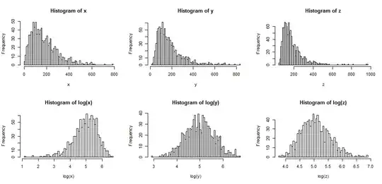
You can see that the center case ($y$) has been transformed to symmetry, while the more mildly right skew case ($x$) is now somewhat left skew. One the other hand, the most skew variable ($z$) is still (slightly) right skew, even after taking logs.
If we wanted our distributions to look more normal, the transformation definitely improved the second and third case. We can see that this might help.
So why does it work?
Note that when we're looking at a picture of the distributional shape, we're not considering the mean or the standard deviation - that just affects the labels on the axis.
So we can imagine looking at some kind of "standardized" variables (while remaining positive, all have similar location and spread, say)
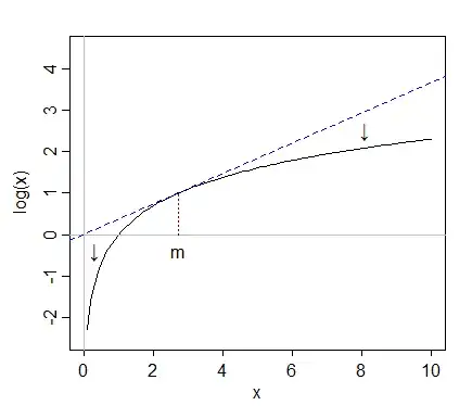
Taking logs "pulls in" more extreme values on the right (high values) relative to the median, while values at the far left (low values) tend to get stretched back, further away from the median.
In the first diagram, $x$, $y$ and $z$ all have means near 178, all have medians close to 150, and their logs all have medians near 5.
When we looks at the original data, a value at the far right - say around 750 - is sitting far above the median. In the case of $y$, it's 5 interquartile ranges above the median.
But when we take logs, it gets pulled back toward the median; after taking logs it's only about 2 interquartile ranges above the median.
Meanwhile a low value like 30 (only 4 values in the sample of size 1000 are below it) is a bit less than one interquartile range below the median of $y$. When we take logs, it's again about two interquartile ranges below the new median.
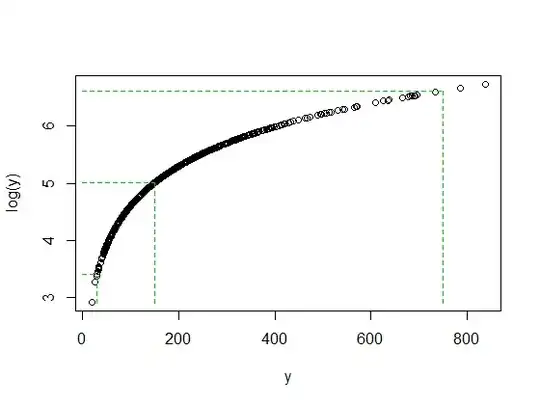
It's no accident that the ratio of 750/150 and 150/30 are both 5 when both log(750) and log(30) ended up about the same distance away from the median of log(y). That's how logs work - converting constant ratios to constant differences.
It's not always the case that the log will help noticeably. For example if you take say a lognormal random variable and shift it substantially to the right (i.e. add a large constant to it) so that the mean became large relative to the standard deviation, then taking the log of that would make very little difference to the shape. It would be less skew - but barely.
But other transformations - the square root, say - will also pull large values in like that. Why are logs in particular, more popular?
I touched on one reason just at the end of the previous part - constant ratios tend to constant differences. This makes logs relatively easy to interpret, since constant percentage changes (like a 20% increase to every one of a set of numbers) become a constant shift. So a decrease of $-0.162$ in the natural log is a 15% decrease in the original numbers, no matter how big the original number is.
A lot of economic and financial data behaves like this, for example (constant or near-constant effects on the percentage scale). The log scale makes a lot of sense in that case. Moreover, as a result of that percentage-scale effect. the spread of values tends to be larger as the mean increases - and taking logs also tends to stabilize the spread. That's usually more important than normality. Indeed, all three distributions in the original diagram come from families where the standard deviation will increase with the mean, and in each case taking logs stabilizes variance. [This doesn't happen with all right skewed data, though. It's just very common in the sort of data that crops up in particular application areas.]
There are also times when the square root will make things more symmetric, but it tends to happen with less skewed distributions than I use in my examples here.
We could (fairly easily) construct another set of three more mildly right-skew examples, where the square root made one left skew, one symmetric and the third was still right-skew (but a bit less skew than before).
What about left-skewed distributions?
If you applied the log transformation to a symmetric distribution, it will tend to make it left-skew for the same reason it often makes a right skew one more symmetric - see the related discussion here.
Correspondingly, if you apply the log-transformation to something that's already left skew, it will tend to make it even more left skew, pulling the things above the median in even more tightly, and stretching things below the median down even harder.
So the log transformation wouldn't be helpful then.
See also power transformations/Tukey's ladder. Distributions that are left skew may be made more symmetric by taking a power (greater than 1 -- squaring say), or by exponentiating. If it has an obvious upper bound, one might subtract observations from the upper bound (giving a right skewed result) and then attempt to transform that.
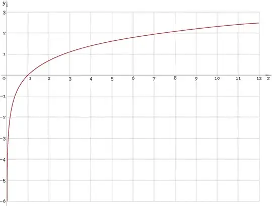
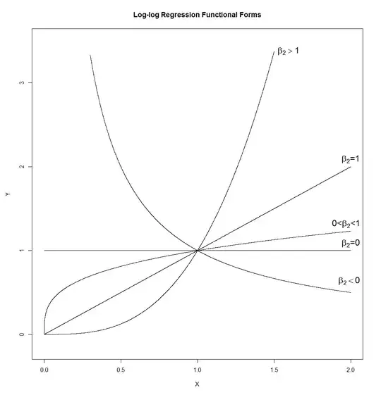 That's a lot of different shapes. A line (whose slope would be determined by $\exp{\left(\beta_1\right)}$, so which can have any positive slope), a hyperbola, a parabola, and a "square-root-like" shape. I've drawn it with $\beta_1=0$ and $\epsilon=0$, but in a real application neither of these would be true, so that the slope and the height of the curves at $X=1$ would be controlled by those rather than set at 1.