whether and to what degree precipitation is correlated with the likelihood of individual congresspeople being present or absent.
There are several options to do this through looking at correlations. One way would be to theorize that underneath both binary variables are latent normal random variables. For example, the attendance latent variable could correspond to willpower to attend projected to $\mathbb{R}$. Then you could find the correlation between these two latent variables in the normal sense. This is the method of polychoric correlation. The R package polycor does this. An example taken from the manual:
set.seed(12345)
data <- rmvnorm(1000, c(0, 0), matrix(c(1, .5, .5, 1), 2, 2))
x <- data[,1]
y <- data[,2]
cor(x, y) # sample correlation
x <- cut(x, c(-Inf, .75, Inf))
y <- cut(y, c(-Inf, -1, .5, 1.5, Inf))
polychor(x, y, ML=TRUE, std.err=TRUE)

#Polychoric Correlation, ML est. = 0.5231 (0.03819)
#Test of bivariate normality: Chisquare = 2.739, df = 2, p = 0.2543
#
#  Row Threshold
#  Threshold Std.Err.
#   0.7537  0.04403
#
#  Column Thresholds
#  Threshold Std.Err.
#1   -0.9842  0.04746
#2    0.4841  0.04127
#3    1.5010  0.06118
You can see it gave you (1) the ML estimate of the correlation with standard error and (2) the threshold estimates for the latent standard normal random variable and their standard errors. This is one approach.
The null hypothesis would be that there is no relationship between precipitation and attendance.
You could test this hypothesis using the correlation above, or you could take a more comprehensive approach and include the other controls you mentioned (amount of precipitation, the temperature, the pressure, lots of weather measurements). This can be accomplished through logistic regression, probit regression, or any other binary regression approach which gives you an understanding of error.
For example, here's some fake data made in R:
set.seed(1932403)
rain = rbinom(1000, 1, 0.2)
rain = (rain == 1)
temp = rnorm(1000)
z = 3 + -2*rain + -1*temp
pr = 1/(1+exp(-z))
attend = rbinom(1000,1,pr)
df = data.frame(attend=attend, rain=rain, temp=temp)
head(df)

#  attend  rain       temp
#1      1  TRUE -1.5418903
#2      1 FALSE  0.2950457
#3      1 FALSE -1.0759618
#4      1 FALSE  0.1218176
#5      1 FALSE -1.1599080
#6      0 FALSE  0.8309843

table(rain, attend)/1000
#       attend
#rain      0   1
#  FALSE  42 757
#  TRUE   63 138
So we can build a logistic model to test if the precipitation is important after controlling for temperature.
m = glm( attend ~ rain + temp, data=df, family="binomial")
summary(m)

#Coefficients:
#            Estimate Std. Error z value Pr(>|z|)
#(Intercept)   3.3835     0.2003  16.890  < 2e-16 ***
#rainTRUE     -2.5190     0.2508 -10.043  < 2e-16 ***
#temp         -1.0918     0.1367  -7.985 1.41e-15 ***
#---
#Signif. codes:  0 ‘***’ 0.001 ‘**’ 0.01 ‘*’ 0.05 ‘.’ 0.1 ‘ ’ 1
And in this fake data it is.
Chances they will be absent, given the fact it's raining?
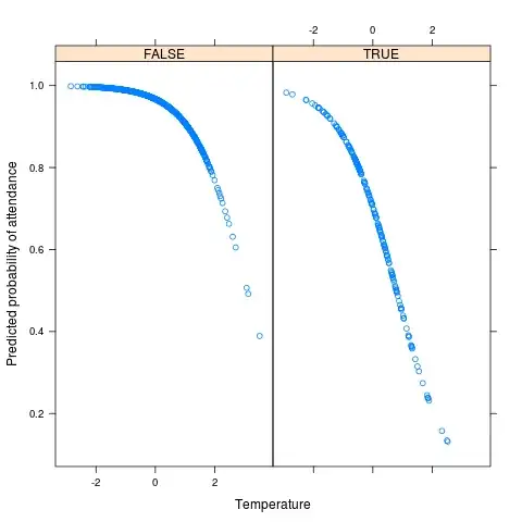
You can plot (and of course, otherwise examine) the predicted probabilities using the model we just built. That is, you can look at the predicted probabilities under different conditions* (here 'TRUE' refers to rain being present):
library(lattice)
xyplot(predict(m, df, type = 'response') ~ df$temp | factor(df$rain), ylab = 'Predicted probability of attendance', xlab = 'Temperature')
Taking a Bayesian approach won't alter the framework you're trying to achieve: predict/build a statistical model around the probability of attendance given certain conditions (rain, temperature, etc.). There are lots of reasons to consider a Bayesian analysis, but none of them stand out as specific to your exact problem.
Another approach (naive to other controls like temperature) would be to do a proportion test.