Regression that creates $x \log(x)$ functions?

Question

I just saw this website, that offers different online regression tools. For example it offers linear regression that creates a function in the form $y=ax+b$. Or it offers power regression that creates a function of the form $y=cx^a$. Or even it provides logarithmic regression that produces a function $y=c\cdot\log(x) +b$.

Now, for a project I am doing, I must find functions in the form $y=c\cdot x\cdot\ln(x)+ b$. Is there any model that can do that? Also is there any tool available like the website I mentioned that offers this kind of regression?

Answer 1

It's quite straightforward.

Simply create a new variable, $x_1 = x\ln(x)$ then fit a linear regression $E(y)=b+cx_1$.

Here's an example (the code is in R but I'll give the data I generate so you can try it in your favourite line-fitting routine):

#generate some data:
set.seed(29384702)
x = runif(20,.05,6)
y = 11.-0.5*x*log(x)+rnorm(20)
plot(x,y)

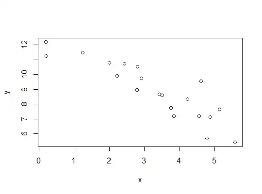
Here's the data (rounded):

    x      y
2.7994 10.536
2.9113  9.748
4.7754  5.681
3.4272  8.663
4.2275  8.347
5.5773  5.404
0.2158 11.270
4.8779  7.118
5.1431  7.634
4.6209  9.550
2.0105 10.805
2.2227  9.918
1.2500 11.497
3.5105  8.611
0.1927 12.197
4.5592  7.179
3.7578  7.755
2.4346 10.739
3.8396  7.204
2.7911  8.978

So as I said, we make a new x-variable:

x1 = x*log(x)

This makes the relationship linear in $x_1$:

and fit what is now linear regression:

yxfit = lm(y~x1)

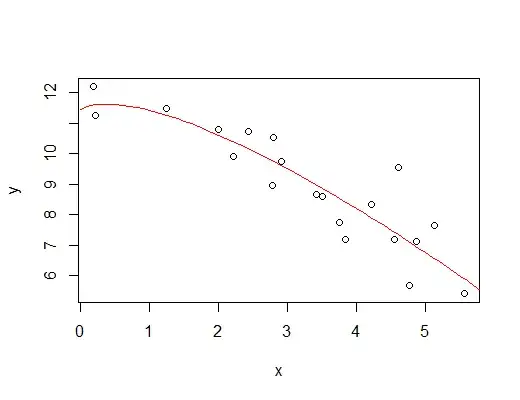
Now let's plot that fitted curve:

xnew = seq(0.01,6.01,.1)
newx1 = data.frame(x1=xnew*log(xnew))
predyx = predict(yxfit,newdata=newx1)
lines(predyx~xnew,col=2)

producing:

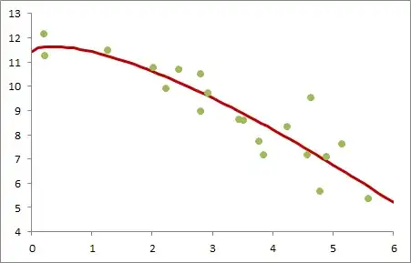
We can do it as easily in something else. Here's a plot of the result of fitting the same model in Excel:

---

Other functions of $x$

The same trick works for any functional fit of the form $E(y)=b+cg(x)$, by letting $x_1=g(x)$.

A much wider variety of functions can be generated by considering models of the form $E(y)=\beta_0+\beta_1f_1(x)+\beta_2f_2(x)+...+\beta_kf_k(x)+\varepsilon$, which may be fitted by ordinary multiple regression as long as care is taken to avoid multicollinearity.

You may be interested to see here where a sinusoidal model, and then a more complicated periodic model are fitted using linear regression.

---

One thing you should be aware of with fitting curved models, such as fitting a function of the form $ax^b$ say, is the assumption about the variation of the points about the mean; it can affect the suitability of some of those choices of model - at least for some purposes - as well as the efficiency of the estimates. Whenever the $y$ variable is transformed to linearize a model you change the assumptions you make about the variation about the model (and note also that if your fit is approximating the expected value on the transformed-y scale, when you transform it back, it's no longer an expectation).

You should make sure that what is being done to fit the model makes sense for your data.