1) A plot of residuals against $y$ will always show a correlation (unless the predictor is perfectly useless). See here and here.
2) On the other hand, the appearance of downsloping lines in your last plot are a direct result of the fact that your $y$ is discrete.
3) The fact that $y$ is discrete isn't necessarily a concern. It seems to me there is a related concern though - in that years of education is effectively bounded, and that means as you approach the bounds a linear fit may be biased. There's a slight indication of that at the low end of your fit. If that small bias is enough for you to worry about, you'll need to do something about it. It also has tendency to cause heteroskedasticity, but there's not strong indication of that here.
The bias is actually very small, so it may not be much of a problem:

The effective lower bound of 12 years of education produces this small bias, as the linear model plows straight through the bound, while (as the loess shows), the local relationship flattens out.
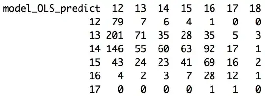
Your table illustrates something else you expect to see - regression to the mean. That table is giving you a misleading impression of the quality of your model, by confounding two different effects (one you want to try to avoid, but which is small in impact, and one you almost surely don't want to avoid).
Consider this linear model (which has no bias from any boundary):

Looking at rows and columns of your table is like taking horizontal and vertical slices in the plot. The regression should give you an approximately unbiased relationship in slices of the fitted (the red $y=x$ line is near the middle of the green slice), but won't (and should not!) give you an unbiased fit the other way (the blue slice). If you look at the blue slice, all the points are to the left of the line.
If you sliced my points up into squares like yours (sliced in the blue and green directions), my table would look a lot like yours. That's not a problem with the model - my model was the one that generated the data.
As for how to deal with the small bias you do have from the lower boundary -
You might try, for example, a logistic model limited to 12-18 (or some larger value for the upper bound, if you can find an effective upper limit that would apply more broadly than your sample; 20 may do better than 18, for example, but you may be able to inform it by external information), or any of a variety of other nonlinear models that incorporate a lower bound (there are many such functions in common use).
So that would involve using nonlinear least squares.
Another possibility is to fit some smooth function - indeed that's exactly what you have already with your loess curve. What's wrong with using that fit? Spline curves could work; but you would probably want to use natural splines with only a few knots, all down the left end (you may even want to force it to be horizontal at the extreme left, but if you do that you might as well go to the nonlinear regression I started with)