Pages 13-20 of the tutorial you posted provide a very intuitive geometric explanation of how PCA is used for dimensionality reduction.
The 13x13 matrix you mention is probably the "loading" or "rotation" matrix (I'm guessing your original data had 13 variables?) which can be interpreted in one of two (equivalent) ways:
The (absolute values of the) columns of your loading matrix describe how much each variable proportionally "contributes" to each component.
The rotation matrix rotates your data onto the basis defined by your rotation matrix. So if you have 2-D data and multiply your data by your rotation matrix, your new X-axis will be the first principal component and the new Y-axis will be the second principal component.
EDIT: This question gets asked a lot, so I'm just going to lay out a detailed visual explanation of what is going on when we use PCA for dimensionality reduction.
Consider a sample of 50 points generated from y=x + noise. The first principal component will lie along the line y=x and the second component will lie along the line y=-x, as shown below.
The aspect ratio messes it up a little, but take my word for it that the components are orthogonal. Applying PCA will rotate our data so the components become the x and y axes:
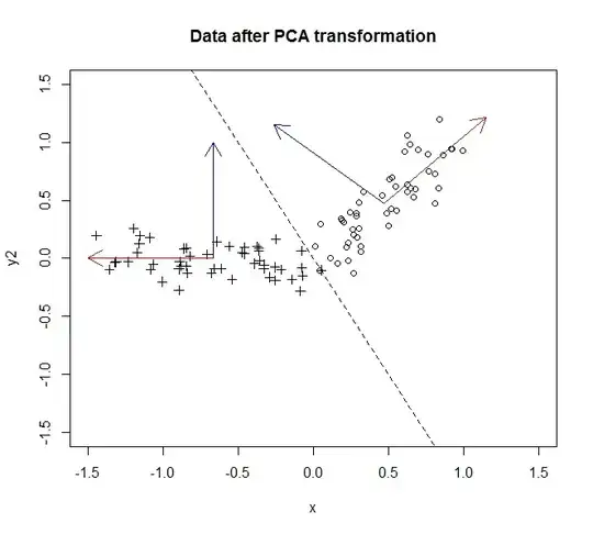
The data before the transformation are circles, the data after are crosses. In this particular example, the data wasn't rotated so much as it was flipped across the line y=-2x, but we could have just as easily inverted the y-axis to make this truly a rotation without loss of generality as described here.
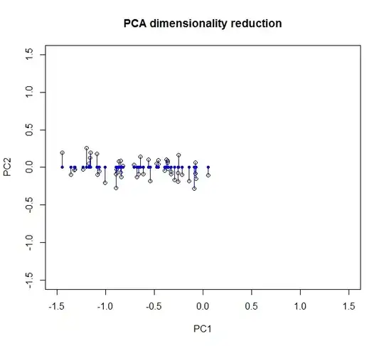
The bulk of the variance, i.e. the information in the data, is spread along the first principal component (which is represented by the x-axis after we have transformed the data). There's a little variance along the second component (now the y-axis), but we can drop this component entirely without significant loss of information. So to collapse this from two dimensions into 1, we let the projection of the data onto the first principal component completely describe our data.
We can partially recover our original data by rotating (ok, projecting) it back onto the original axes.
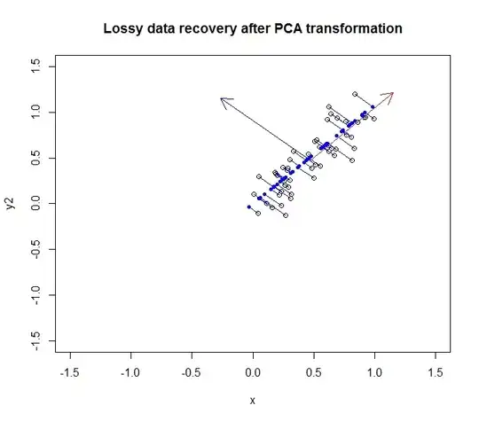
The dark blue points are the "recovered" data, whereas the empty points are the original data. As you can see, we have lost some of the information from the original data, specifically the variance in the direction of the second principal component. But for many purposes, this compressed description (using the projection along the first principal component) may suit our needs.
Here's the code I used to generate this example in case you want to replicate it yourself. If you reduce the variance of the noise component on the second line, the amount of data lost by the PCA transformation will decrease as well because the data will converge onto the first principal component:
set.seed(123)
y2 = x + rnorm(n,0,.2)
mydata = cbind(x,y2)
m2 = colMeans(mydata)

p2 = prcomp(mydata, center=F, scale=F)
reduced2= cbind(p2$x[,1], rep(0, nrow(p2$x)))
recovered = reduced2 %*% p2$rotation

plot(mydata, xlim=c(-1.5,1.5), ylim=c(-1.5,1.5), main='Data with principal component vectors')
arrows(x0=m2[1], y0=m2[2]
       ,x1=m2[1]+abs(p2$rotation[1,1])
       ,y1=m2[2]+abs(p2$rotation[2,1])
       , col='red')
arrows(x0=m2[1], y0=m2[2]
       ,x1=m2[1]+p2$rotation[1,2]
       ,y1=m2[2]+p2$rotation[2,2]
       , col='blue')

plot(mydata, xlim=c(-1.5,1.5), ylim=c(-1.5,1.5), main='Data after PCA transformation')
points(p2$x, col='black', pch=3)
arrows(x0=m2[1], y0=m2[2]
       ,x1=m2[1]+abs(p2$rotation[1,1])
       ,y1=m2[2]+abs(p2$rotation[2,1])
       , col='red')
arrows(x0=m2[1], y0=m2[2]
       ,x1=m2[1]+p2$rotation[1,2]
       ,y1=m2[2]+p2$rotation[2,2]
       , col='blue')
arrows(x0=mean(p2$x[,1])
      ,y0=0
      ,x1=mean(p2$x[,1])
      ,y1=1
      ,col='blue'
       )
arrows(x0=mean(p2$x[,1])
       ,y0=0
       ,x1=-1.5
       ,y1=0
       ,col='red'
)
lines(x=c(-1,1), y=c(2,-2), lty=2)


plot(p2$x, xlim=c(-1.5,1.5), ylim=c(-1.5,1.5), main='PCA dimensionality reduction')
points(reduced2, pch=20, col="blue")
for(i in 1:n){
  lines(rbind(reduced2[i,], p2$x[i,]), col='blue')
}

plot(mydata, xlim=c(-1.5,1.5), ylim=c(-1.5,1.5), main='Lossy data recovery after PCA transformation')
arrows(x0=m2[1], y0=m2[2]
       ,x1=m2[1]+abs(p2$rotation[1,1])
       ,y1=m2[2]+abs(p2$rotation[2,1])
       , col='red')
arrows(x0=m2[1], y0=m2[2]
       ,x1=m2[1]+p2$rotation[1,2]
       ,y1=m2[2]+p2$rotation[2,2]
       , col='blue')
for(i in 1:n){
  lines(rbind(recovered[i,], mydata[i,]), col='blue')
}
points(recovered, col='blue', pch=20)